1.2 Introduction to Statistics
1 Statistical Models
A statistical model is a family
Suppose
- Model 1: all flips are independent, with
. Then , with So . - Model 2: flippers have different same-side biases, and are independent.
, . - Model 3: Biases get smaller over time,
. May add a constrain .
1.1 Parametric vs Nonparametric Models
Parametric models are distributions indexed by
Denote
On the contrary, non-parametric models means no natural way to parameterize
Simple case for non-parametric models is
, is ANY distribution on . Then , .
However, we can use "parametric notation"
1.2 Bayesian vs Frequentist Inference
So far we assume data
This helps reduce the problem of inference, and we can focus on the conditional distribution of
However, before introducing Bayesian Inference, we assume
2 Estimation
We want to determine the value of a parameter in a parametric model.
- Skeptical answer: could be anything.
- Bayesian answer: assume
random with prior distribution, and calculate conditional distribution of . - Frequentist answer: inductive behavior: find a method for using
to estimate . E.g. . Show it generally works well for every .
General step:. Estimate . Observe , calculate estimate using .
Loss function
E.g., square error loss
.
Risk function is the expected loss of an estimator:
For square error loss, it is called mean square error (MSE):
In brief, we have two primary strategies to choose an estimator:
- Summarize the risk function by a scalar.
- Restrict attention to a smaller class of estimators.
Suppose we stick to model 1 in here. For
We can show several estimators: 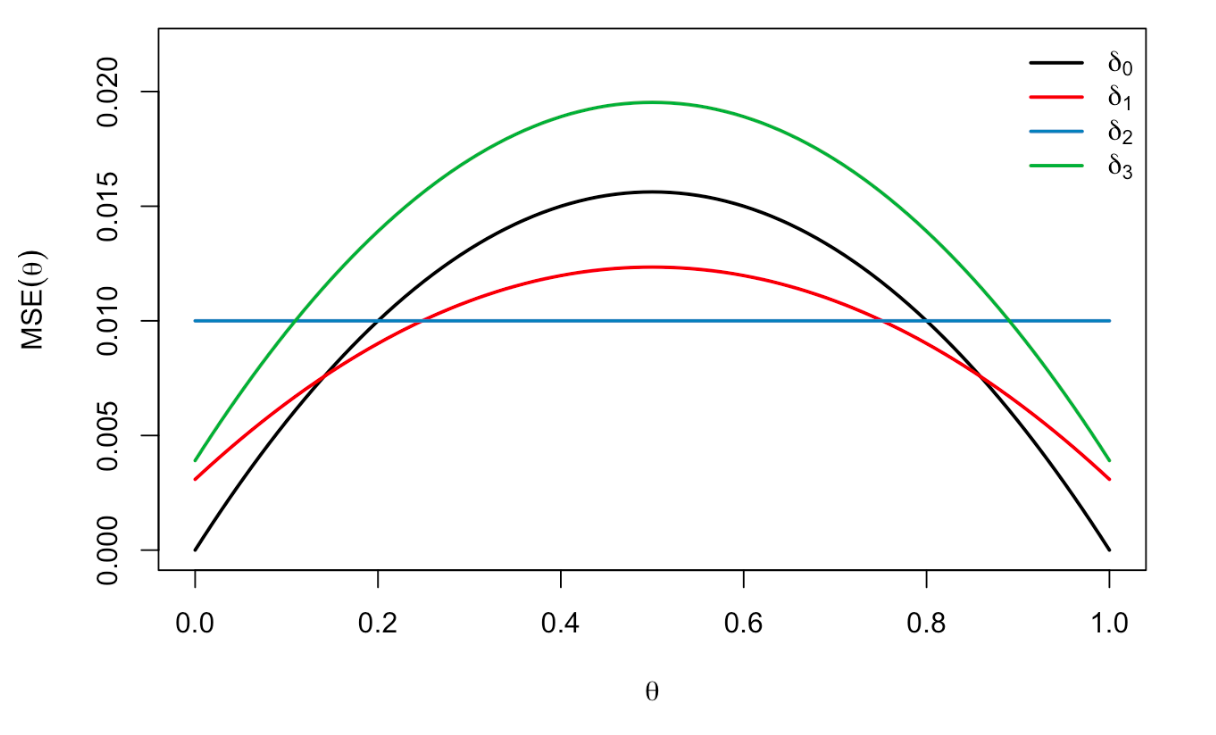
Compared with
2.1 Comparing Estimators
An estimator
; .
We say
2.2 Resolving Ambiguity
There is no estimator that uniformly attains the smallest risk among all estimators. Like the brute
Summarize the risk function by a scalar.
- Average-case risk (Bayes estimation): minimize some (weighted) average of the risk function over
:
If, we can assume WLOG that is a probability measure. Then this average is the same as called the Bayes risk. An estimator minimizing the Bayes risk is called the Bayes estimator. - Worst-case risk (Minimax estimation):
This will push us to choose estimators with flat risk functions, like from the example.
Restrict the choice of estimators
Unbiased estimation: we can demand an estimator to satisfy
Under unbiasedness, we can clearly define the optimal estimator called UMVU estimator. From the above example,